If you’re not yet familiar with the VLOOKUP and HLOOKUP functions, you’re definitely missing a valuable tool in your toolbox! These two functions enable highly efficient searches and automate many processes. That said, like all Excel functions, these are most interesting when used in combination with other functions, such as MATCH.
What is the purpose of the VLOOKUP and HLOOKUP functions?
The VLOOKUP function (vertical search)
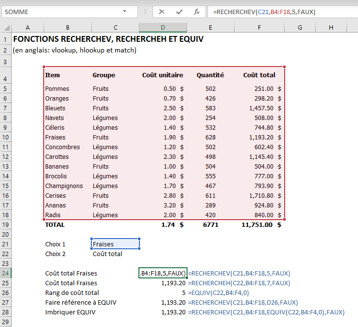
The VLOOKUP function allows you to search for a value in the first column of a data table and extract another value, in the same row, in the column of your choice. More precisely, the parameters are defined as follows:
- Desired value
- Table in which we search for the value
- Column from which to extract the corresponding value
- TRUE/FALSE (False assumes an exact match, otherwise the formula returns an error message)
So, below, we look for the item STRAWBERRIES, in the red table, and then ask you to return the value of the 5th column on the strawberries line, which corresponds to the TOTAL COST. The result is $1,193.20.

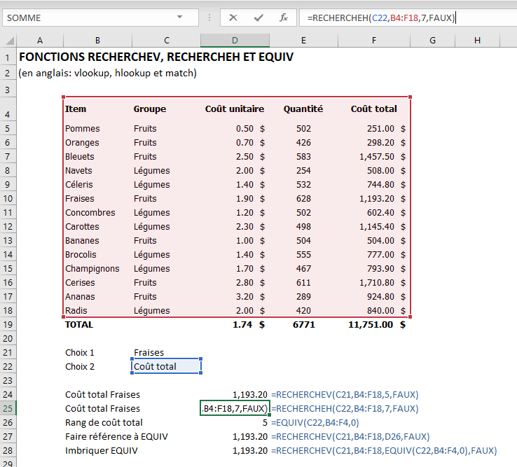
HLOOKUP (horizontal search) function
The HLOOKUP function is identical to the previous function, except that it searches for a value in the first row of a table and returns a value in that same column, in the row of your choice. So, below, we search for the TOTAL COST header, in the red table, and return the value of the 5th line, the strawberry line, which also returns $1,193.20. Here, therefore, it is possible to obtain the total cost of milling cutters using both the VLOOKUP and HLOOKUP functions.
The dangers of VLOOKUP and HLOOKUP functions
Impact of adding a column
If someone uses your file and adds a column, then inserts new information, the total cost searched by function VLOOKUP will no longer be in the 5th column, but rather in the 6th column. By doing so, you’ll get not the total cost but rather the quantity, i.e. 628.

Impact of adding a line
Similarly, if you had used the VLOOKUP function and a colleague added a new line to your file, your HLOOKUP formula would return the total cost of the CELEBRATES rather than the COSTS, since the CELEBRATES would then be on line 6. The strawberries would then be on line 7.

The great utility of the MATCH function
It’s in situations like these that we begin to understand the full benefits of the MATCH function. In fact, as long as a function requires a column or row number as a parameter, your function is at risk and can quickly go off the rails by adding rows or columns. This is why it’s very useful to replace the row or column number with an MATCH function, which will naturally return the correct number.
More precisely, the MATCH function is used to find out the rank of a value in a column or row. This involves providing the following parameters:
- Desired value
- Row or column in which to search for the value
- 0, 1, -1 (0 means an exact match)
So, below, we search TOTAL COST in the row representing column titles and ask you to return the column number, which is 5.

The robustness of function nesting
You can then link the column number of function VLOOKUP or the row number of function HLOOKUP to this MATCH function. Below, we’ve replaced the 5, which was a manually-entered value, with reference D26, which includes the MATCH function, which itself returns a 5 but will become 6 if we add a line to the file or 7 if we add 2, and so on.

It would also be possible to nest the MATCH function inside the VLOOKUP function to avoid having to produce 2 steps in two different cells to arrive at the same result.

In this case, it’s clear from the image below that adding a new column wouldn’t affect the function in any way, which would continue to return $1,193.20, the total cost of the strawberries (compared with the function VLOOKUP, which no longer returns the correct amount).
Likewise, we can see that adding a new line would not affect the reported result either, whereas the HLOOKUP function produces an error.
What’s more, the user can easily change the item to search for and the column header to search in, and still get the right result. For example, here we’re asking for the unit cost of cucumbers, and functions using the MATCH function return the correct results, while functions VLOOKUP and HLOOKUP return incorrect values.

You may also be interested in the following articles:
Excel: Add multiple tabs with a single mouse click
Excel: The Indirect function for creating executive summaries at the click of a mouse
Excel function: Offset
Excel function: Index/Equiv (Index/Match)
Excel functions: vlookup, hlookup and match
Excel function: Sum.si (sumif)
Excel function: Sumprod (Sumproduct)
Accompanying file
To download the file used in this tutorial, become a VIP member of CFO Masqué.
Further training
To deepen your knowledge of Excel, including data validation, we recommend our training course Excel – Mise à niveau.
Here are a few comments from learners who have taken the Excel – Mise à niveau online training course:

 La mission du CFO masqué est de développer les compétences techniques des analystes et des contrôleurs de gestion en informatique décisionnelle avec Excel et Power BI et favoriser l’atteinte de leur plein potentiel, en stimulant leur autonomie, leur curiosité, leur raisonnement logique, leur esprit critique et leur créativité.